In this project, we create a physics-based ray tracer for rendering 3D scenes. Ray tracing involves calculating the color of objects in much the same way the photosensor of a camera would, or even the eyes of an animal. Light rays from various light sources bounce around a scene, and some of them hit the photoreceptor, creating the various colors and shades on an image. Our ray tracer is similar in that it also simulates the bouncing of light rays around a scene.
Note: Hover over any image for a zoomed in version. Up-scaling is done using nearest-pixel to preserve pixel definition. This can be used to see very small details like edge lines.
So in the real world, light rays are always being produced by energy sources like light bulbs, the sun, and even non-visible sources like remote controls and microwaves. But trying to simulate all of these light rays can be very processor intensive, as many of the light rays may not even enter the virtual camera lens. But there is a property of light that can help fix this problem. Symmetry.
Symmetry states that light rays are bidirectional - that if we have a single photon that bounces around a scene and exits, if we reverse the direction of the photon, we will arrive at exactly where it originated from. This means that rather than simulating real light rays, we can instead generate "camera" rays, or rays from the camera that we expect will hit light sources.
We do this by generating a packet of randomly distributed rays for every pixel we need to render. The random distribution helps to achieve micro-details that our otherwise pixel-perfect screen could not achieve. As the ray exits the camera, we begin intersecting with 3D primitives.
For triangles, we can calculate intersection quite easily. Because a triangle uniquely defines a single plane, we can simply intersect a ray against the plane. When we find this intersection point, we can easily convert into 2D coordinates, interpolating barycentric coordinates to define where on this triangle we hit. If our barycentric coordinates are negative or very large, we immediately know that the ray passes by the triangle, rather than hitting it.
If we intersect, we can evaluate an additional time coordinate. This is used to define the exact contact point. Because we have the ray's origin, and the ray's direction, we can follow the direction vector for some amount of time (the one we just calculated) to determine the contact point.
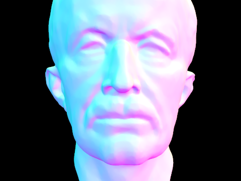
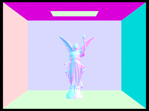
Here we can see the ray-tracer in action. Currently, we render images only by the normal vector of the hit point.
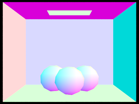


The intersection code for spheres is not much more difficult. Here we have sphere intersection:
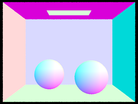
It is important to note that the images above contained varying amounts of triangles, and because our current intersection algorithm is naive in that it just intersects against all primitives in the scene, render times for these simple scenes can be very large.
So we want to speed intersection up. Here's the basic idea. If we shoot a light ray forwards, is it necessary to calculate intersection of primitives that are behind the ray?
Technically we can ignore all primitives that don't intersect the ray. But how efficient is this method? Using Bounding Volume Hierarchy, we can speed intersection calculations by a large amount. The main idea is exactly that calculating ray intersections in front should ignore all primitives behind.
To do this, we construct bounding boxes around groups of primitives intelligently. We note that intersection against a bounding box is very fast. In addition, bounding boxes can be nested such that we can create a large bounding box, and place multiple smaller bounding boxes within that larger bounding box. This is the central idea. So how do we determine which primitives to add to each bounding box?
Well, our objective is to group primitives close together. So the way we do this is we calculate the entire bounding box. we can then split the bounding box in halve against the longest dimension of the bounding box. We do this so that our smaller boxes are roughly cubic, which minimizes the intersection chance by volume (compared to a large very flat box).
We have one safety to catch for. What if all the primitives happen to be on one side of the split axis. Well in this case, we instead take the largest split dimension, and split by median element. Median element is useful in this case because we know that all of the primitives are grouped closely together, so splitting based on the relative locations is better than an arbitrarily defined plane.
With this BVH in place, we can know intersect primitives much more intelligently. We start by intersecting the largest BVH. If our ray does not even hit this BVH, then we already know we can't possibly hit any primitives. If we do, we recurse into this BVH and try intersecting each of it's children BVHs. We recurse all the way to the bottom-most level, where there are a set number of primitives remaining. At this point, we can simply iterate through each primitive and do intersection tests.
With this scheme in place, we can now render scenes with very large amounts of primitives, that we could not render previously.
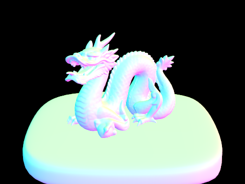
For reference, these scenes took only a dozen seconds or so to render. This is still a relatively large amount of time (considering we haven't even gotten to physics-based light calculations).
So how do we speed it up. This is always the question. Well there are many things we can do.
Let's start by making our BVH more efficient. The method we construct uses a global heuristic which is decent, but not very good. We can improve it by adding a dynamic heuristic. Specifically, we want a heuristic which can find the BVH split that will be the most efficient.
We restart our construction from scratch. Instead, now we try to determine the best way to split these primitives. We define B "buckets" evenly distributed across the x, y, and z axis, with planes dividing each pair of adjacent buckets. What this allows us to do is group the primitives into similar regions based on their centroids.
Why do we do this? Well it turns out that a good estimate of how much computation is needed to evaluate a BVH is the product between the bounding surface area (where rays enter) and the number of primitives within this bounding box. The reason for this is that we take into account both the probability of a ray entering the bounding box, and then how much computation is required to traverse such a BVH.
Now back to the problem. Once we have our split planes, we simply evaluate our heuristic on both sub-BVHs, and the sum is exactly the estimate of how efficient this split is. After iterating through all split planes, and using B=16, we get a pretty good estimate of split planes. Here's a bit of pseudocode:
        function ConstructBVH( primitives[] ):
            for axis x, y, z:
                for each primitive p in primitives:
                    bucket = evaluate_bucket(p.centroid())
                    axis[bucket].expand_bbox(p)
                for each bucket:
                    left, right = split(primitives, bucket)
                    score = left.bbox.surface_area() * left.count_primitives() +
                            right.bbox.surface_area() * right.count_primitives()
            execute split with minimum score
            return BVHNode from split
Now let's test how fast it is now.

We run a few rendering tests on our bunny scene with 28588 primitives. Using the naive method, we average around 7.5 seconds, while using the efficient version, we average 7.4 seconds. However, We construct the BVH in 0.2 seconds for naive, and 0.5 seconds in the efficient algorithm.
Not very impressive it seems. But we realize that is because our efficient algorithm generally provides more speed-up on scenes with many rays, and high primitive count - in other words, complex scenes. Let's test on a more complex one.
We test on the lucy scene, which has 133796 primitives. Using the naive method, we average around 9.27 seconds, while using the efficient version, this drops to only 7.38 seconds! Now that is some real improvement. How does our BVH fair? Well the naive construction takes 1.4 seconds on average, while the efficient construction takes 2.6 seconds.
The amount of time it takes to construct the BVH is independent from rendering times. We realize that the efficient algoithm is very useful for large scenes that require many ray traces. Specifically, rendering a test scene using 256 rays, we get a speed up on the order of minutes, not seconds! On the other hand, the BVH still took the same extra 2 seconds to construct, which is a very good trade-off. This only scales linearly with additional samples, and inverse logarithmically with increasing primitives!
So we have a surface area heuristic to make our BVH more efficient. Can we speed anything up?
Turns out we can. Currently, our entire BVH construction and intersection functions rely on recursion. As we know, recursive processes have a constant factor in speed reduction when compared to equivalent iterative solutions (for the most part). Specifically, our recursive functions are not tail-recursive, and thus every recursion layer, evaluation continually becomes more and more expensive. To solve this, we simply convert to an iterative approach.
Both the construction and intersection methods can be converted in much the same way. First, we construct at the beginning of the function call a std::stack type that will keep track of the remaining primitive groups (for construction) or BVHNodes (for intersection) that we have left to evaluate. Note that this stack is exactly the same idea as a recursive call stack! But instead, we no longer need to keep track of call frames and, as such, we can throw out data in the function we already know we won't need to use.
For example, in our intersection function, we keep track of a hit boolean whenever we intersect a primitive. In a recursive scheme, we execute the following recursive call: [pseudocode]
        function BVHIntersect(BVHNode node):
            hit = node.primitives.intersect(...)
            for left and right of node:
                hit |= BVHIntersect(left) or BVHIntersect(right)
            return hit
This creates an entirely new hit variable for every layer of our BVH! Instead, we only need to keep track of one hit boolean, which allows for using a stack instead for an iterative approach.
        function BVHIntersect(BVHNode node):
            stack = stack(node)
            hit = False
            while nodes remaining and not evaluated in stack:
                hit |= node.primitives.intersect(...)
                add node.left and node.right to stack
            return hit
Additionally, many other variables are saved, reducing memory usage. Since fewer function calls are made, we also save on time in creating each new function frame. So how does the runtime compare?
SPOILERS For this test, we borrow upon one of the images you will see shortly in a later section that uses physics-based rendering. This is because, these scenes tend to be much more processor intensive, and thus it is easier to test asymptotic speed-ups like such.

Using a recursive implementation, it turns out that this scene takes just about 300 seconds on average to render, although sometimes dipping as low as 260 seconds. What about our iterative solution? Rendering times for the dragon take 250 seconds on average, though commonly taking a consistent 230 seconds! This speed-up is great, and it shows how there is a constant factor slowing down recursive approaches (especially with very deep binary trees such as our BVHs.)
There's just one thing left to do. We've made our solution more efficient. We've made it faster. Now all we have left is memory! There are a few ways to do this. For one, we want to use pointers in all situations, and never pass objects such as these by data. Always by reference. Because these BVHNodes contain so much information, passing BVHNodes around causes creating new copies every time. Now this problem mainly existed in the recursive implementation, and has largely been fixed with an iterative approach.
Another memory saving task we can do is to re-compress the tree when we are done. Rather than keeping a vector of primitives, we instead keep track of contiguous chunks of primitives. This saves memory when primitives are near each other, both in the 3D scene, and in their relative positions in memory. In addition, we can further extend this by keeping a single pointer to a specific location in a large list of primitives, along with the number of primitives such a BVHNode has. Instead, we sort the list of primitives such that we can keep a pointer to the starting position in an array, along with the number of elements that we request, and simply iterate as such. This method, however, involves rebuilding the entire tree, which may cause issues when it comes to partitioning efficiently (think about how to make this fast without using exponential time). We will leave memory compression as an exercise for the reader.
There are many other ways we could implement to speed up our rendering times! Unfortunately, some other techniques require much more work that don't show as much improvement for such small scenes as the ones we test. On the bright side, each optimization stacks upon another, and in later parts of the project, we will see that cutting rendering times from 1200 seconds to only 250 seconds (the dragon scene) can save a large amount of heartache (especially when the output image is just black :P).
But enough about optimizations, let's talk about how we made that amazing dragon rendering!
(Finally moving on,) direct illumination. What exactly does it do? Well direct illumination, or direct lighting, is a way of calculating the amount of light a material receives from the surrounding world. We discussed earlier how we can generate images by shooting multiple "camera" rays into the world to test for color, and recombine into a single image. Direct lighting uses the same concept.
Instead, let's take the scenario where we projected many camera rays onto the scene. How do we know what the color of that object is? In normal shading, the color depended only on the normal vector. But now, we want to calculate using real ray-tracing. The solution is simple, we repeat the distribution process, shooting rays outwards from the point of intersection to determine the incoming radiance. We can then use this value to determine how the material will affect the light, and thus solve for an outgoing spectrum!
But we already meet a problem. Light sources are sparse in a 3D world. Most rays we test will result in black, which causes a very speckled rendering. The solution is quite elegant. Note that the scene does not change. This means, using math, given any point on the scene, we can immediately calculate the exact positions of each light in the scene, and the rays that we require to hit them, whether it take one bounce, two bounces, or multiple bounces to reach that light (as we will see in Part 4)!
So instead, we modify our ray-tracing to only trace those rays that will end up hitting a light source. This seems very biased. It is biased! But it's a simple fix. We simply need to determine how much of all rays we could project end up hitting a light source. This ratio of rays that hit lights to rays that don't can be used to scale down our resultant light, and effectively we remove the bias presented earlier.
Let's go back to the dragon rendering.
If we consider any shadow, we can imagine a handful of light rays being cast towards the right side, where an area lamp is present. Specifically, consider the shadow behind the dragon towards the left. When we project our light rays, some of them hit the light, while others end up colliding with the dragon's body. This is why the shadow gets darker in areas that are more difficult in reaching a light source.
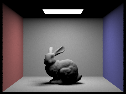
Here's another rendering. This is the same bunny from before.

We only used 8 samples to render this image. What happens when we use more?

Better. Now let's play around with the light rays.


There is a pretty dominant pattern forming. Darker areas which receive little light become more and more refined as the scene is allowed to render with more light rays. Finally, we increase our samples and see how much it impacts.

As you can tell, using 4 times as many samples barely increased quality, while in Fig. 3.2 and Fig 3.3, we can see that the small increase in samples helped much more. So we know that rendering a good scene requires a careful balance between samples and light rays. Preferably, we would even want to use an adaptive sampling strategy. This kind of sampling method instead samples a small fixed number of times, and then tests the variance between samples of each pixel. If the variance is greater than some threshold that we arbitrarily set, then we continue rendering more samples. This allows for the image to "fix" itself in noisier areas.
Even better, we can define a dynamic variance threshold intelligently if we know we are rendering an area of high contrast (say the edge of a sphere or interface between two materials).
Anyhow, even with direct lighting, our scenes aren't particularly realistic. Let's see how we can improve on that.
Indirect lighting is similar to direct lighting. The difference, however, is that rather than calculating rays towards lights, we instead calculate rays towards the surrounding scene, and then bounce to light sources. This allows us to pick up reflections, diffuse color, and other sources that we weren't able to collect earlier.
The main idea is that when we intersect a primitive, we instead cast light rays in some direction dependant on the material. For example, a diffuse material would scatter light uniformly, while a mirror material would reflect on the exact opposite ray. We can then trace this ray and determine the resultant color, adding it onto the current intersection fragment.
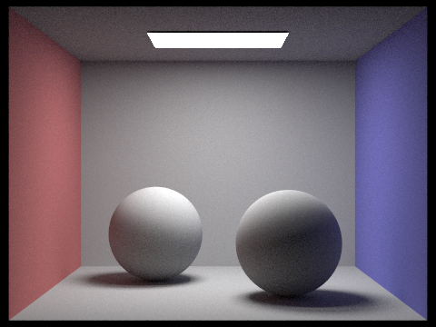
Here we have a few images rendered using global illumination:


Note specifically the color bleeding along the edges of walls. This is due to the indirect illumination picking up colors as rays bounce around the scene.
Let's see what indirect lighting is really doing. We can separate out the direct and indirect lighting and see what our rays actually "see".
We will start with a direct lighting image, and then the corresponding indirect lighting at various ray bounces. Note that all renderings are rendered with 16 samples and 16 light bounces, so differences will only be in the number of ray bounces.


We can see an obvious pattern forming: first bounce is generally the light we see from light reflected off of the floor and walls. The second bounce is the light reflected off of the bounce from the first. The third is the same, except using the second, and so forth. Note that the longer a ray bounces, the darker that ray gets. We introduce a new concept.
Russian roulette is a method of terminating indirect illumination ray bounces. If we can't terminate bounces, then we'll end up calculating many pointless rays that contribute little to no light to the overall scene. Russian roulette instead terminates light rays that are too dark to have any meaningful contribution to the scene.
We can see it's affect. Now we will render scenes with cumulative indirect lighting. Cumulative will add the first n ray bounces of light, discarding the first bounce (as that is direct lighting).


There is an obvious pattern. Seeing as in Fig. 4.7, light contribution decreases, it is easy to guess that if we calculated the 16th ray bounce, we'd get a pure black screen, due to all rays being destroyed before returning a color. What does that imply about using 16 ray bounces?
The 16th ray bounce will have "converged" towards the true color. At this point, increasing ray bounces to a ridiculous amount would have little to no affect.

So we can tell what indirect illumination looks like. Let's combine the two and compare differences.
We've done enough bunnies. Let's turn to spheres. Here we will test the same theory as above - changing the number of ray bounces. All renderings are rendered at 64 samples per pixel for HD, and 8 light samples.


As expected, more ray bounces converge towards the final image. Again, we render a 32 ray bounce and show that there are minimal differences, meaning that light rays are converging.

What about sample rate. How does that affect indirect illumination?
Sample rate, in general, affects the quality of the entire image, and thus we should see similar results as those between Fig. 3.2 and Fig. 3.3.
Here, we render images at 8 light samples, and 5 ray bounces. We change the samples per pixel only.


As expected, our images also converge. However, we note that they converge much slower. This is due to the fact that areas of high variance (as stated earlier after adaptive sampling discussion) tend to take longer to average out. We see this specifically in dark corners, where a sample of light might return pure black, or pure white. This ends up magnifying the speckled result when probabilistically we hit more lights on some samples, and less lights with others.
Finally, at 1024 samples, we have HD renderings that should approach convergence.

Phew! Now that is what we call a photo dump! Let's move onto the last part where we mess around with various materials.
Recall that a material can define the way light reflects off of the surface of a material, along with other attributes it changes, like color and luminance. Here, we start by creating a very simple material.
This material is a mirror material. When a light vector hits this type of material, we request the exact reflection vector to render. This results in pure, non-glossy reflections.
In addition, we can define a color for the mirror. The following dragon is rendered with a gold mirror color, and non-glossy pure reflections.

Note that the reflection along left-facing faces have the red tinge of the wall, while reflections on the right-facing faces have a blue tinge. In addition, the lamp can be seen reflecting only off of a very specific portion of the dragon's body (as opposed to the entirety of upper-facing faces.
We can define another material that simulates glass. Glass has two main properties we should be concerned with:
Thus, we can first create a refractor. Refracted light rays are evaluated by taking the ratio of the index of refraction between two materials, and bending the angle of the light towards or away from the normal depending on this ratio. The index of refraction defines how "dense" or how much "slower" light travels through the medium. In reality, the speed of light remains constant, and instead it's perceived as slower because of how densely packed atoms are, scattering light and thus increasing the effective distance it must travel through such a medium.
Once we've calculated the new light ray, we can move onto evaluating the Fresnel factor. Fresnel equations tell us the proportion between light energy being reflected and refracted. We can estimate the Fresnel equations using Shlick's approximation. In this way, we can determine exactly how much reflection we should see.
In the end, we simply reflect light whenever total internal refraction occurs. If not, we evaluate the Fresnel equations to get a ratio between reflection and refraction. We then randomly choose one with probability dependent on the ratio so as we reach infinite samples, our ratio converges.
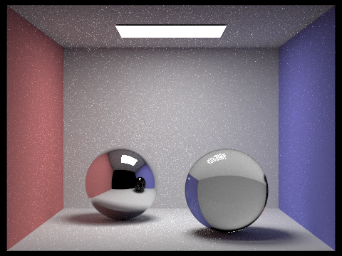
Let's see some images of varying ray depths. The following images are rendered at 64 samples and 16 light bounces. The left sphere uses a mirror shader, while the right sphere uses a glass shader.
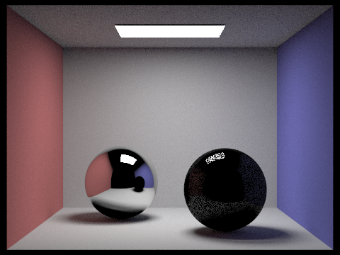
We note two things. First, the refraction sphere is nearly black. This is because most light rays refract and, since this counts as a bounce, terminate after entering the sphere. Another interesting note is that the mirror returns a black color for the ceiling. This is the same reason why refraction turns out to be black.
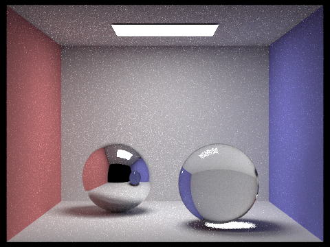
With two ray bounces, we get some improvement. The refraction now shows up correctly. However, for the same reason, the reflection of the right sphere in the left sphere turns out black because we have spent two ray bounces reaching the ball, and terminate before exitting the sphere.
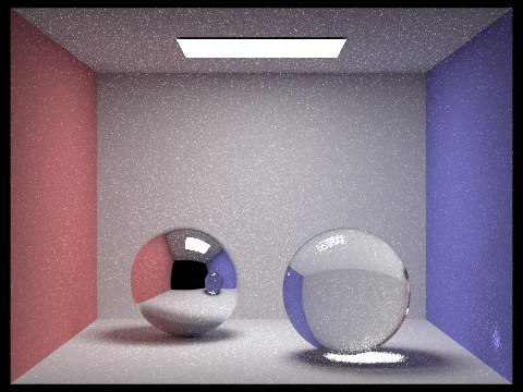
With the third bounce, we fix the reflection of the dark sphere. Furthermore, we note that light passing through the glass sphere now successfully hits the floor.

Note the light ray that manages to hit the right wall. We will speed through the remaining bounces.

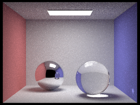

We can see that with each increasing light bounce, we increase the chance of light scattering and hitting some wall. The glass sphere surface, for example, now has a bright area. The scene is also generally brighter due to the increased amount of light bouncing.
So what happens when all the light bounces converge into blackness using Russian Roulette? Well this is the final image we get, using 256 ray bounces.

As you can see, not much changed. There's a new reflection at the top right area on the ceiling, and some of the caustics become more apparent.
Now what happens if we increase the sample rate. We can tell that even with 64 samples, the images are still speckled. This is because mirror and glass types take much longer to converge. So now we will test how sample amount affects our scene. We will render with 1 light sample, and 256 ray bounces so we can reach convergence.

As expected, with one sample, our scene is very very speckled.


As we can tell, the speckles are still apparent with 64 samples. This is, again, due to the slower convergence of sample rate, and the addition of glass BRDFs. We render at 1024 samples and see that the scene is slightly fixed.

There are lots of other materials we could implement for additional amusing results. But seeing as the series of spheres took a total of an hour to render, we'll leave more complex materials as an exercise for the reader.
What other fun things can we add? Well for one, we can simulate a real camera with an aperture. This allows us to mess with factors like depth of field. How do we do this?
Well first we need to understand what a camera aperture even does to a camera. In our current "pinhole camera" version, all rays originate from the same point. This means we can calculate the exact ray that projects to some pixel on the screen. However, in a real camera, there is a lens that gathers light and channels that light onto a sensor plate. The difference is that the aperture on a real camera has some non-negligible radius that gathers rays of light from more than one location.
Ultimately, this means that when rendering a screen pixel, simulating a real camera involves taking samples across that lens to simulate the aperture size. We can do this easily.
First we start by defining a focal point. For our version, we used the targetPos as the focal point. Then, we will move our projection plane to that focal point. This means that we need to change the width and height of our sensor plate so that the projected image is still the same size.
Next, we add support for simulating a camera aperture. We can do this by taking samples uniformly distributed along a disc. Alternatively, we could generate points along a fixed polygon like a pentagon or hexagon to further simulate the aperture shape :D. Afterwards, we simply displace the origin of the vector.
Because we've displaced the origin, we also need to account for the change in direction, since we need the vector to still hit the correct pixel (otherwise all we've done is blur the image a lot). Finally, rendering the image, we now have a easy way to focus on different objects. Let's see what we can do with it.
In the following images, we render at 64 samples per pixel, with 1 light sample and 256 ray bounces. We test various aperture radius and see the outcome.


Finally let's re-render that last image with 1024 samples instead.

Any maybe try that last one with a 0.15 radius lens.

Unfortunately, as visible in the last two, adding depth of field causes higher error (which we can use adaptive sampling to fix), which means we need more samples in order to render a similar quality image.
Just because depth of field is fun to play with, here's a rendering of a dragon :D.

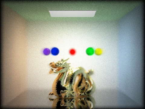
The focus is very fun to play with. So fun that we ended up modifying one of the render files (the dragon one) to render some decent images. Here they are.
In each image, we changed the floor to be a silver mirror. We then changed the color of the surrounding walls. Finally, we added 5 glass spheres with the IOR of water. These are the output images. In addition, a post-processing algorithm was applied to each render to enhance the image. The first involved using a sliding filter to progressively blur and overlay the image outwards from the center. This reduced speckles. The second took areas of high luminance, and white-washed the colors, followed by subtly blurring. This gave bright areas a glowy feel. Finally, a simple ovular vignette was applied. This was generated by simply creating a mask buffer containing a circle, then scaling to interpolate until the correct ovular shape was found, and finally blurring and multiplying the output color with the image.

Thanks for reading! I hope you enjoyed all of the images.